
| Channel | Publish Date | Thumbnail & View Count | Actions |
|---|---|---|---|
 Rabi Gurung Rabi Gurung | 2023-06-05 13:00:39 | 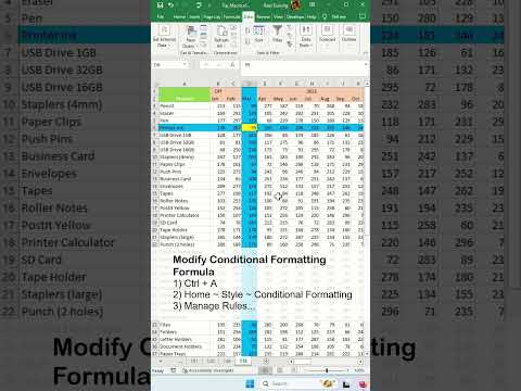 11,551 Views |
Now you know how to crosshair highlight in excel, essentially, how to highlight row and column of active cell. And also create a crosshair highlight with intersecting cell as a different colour. The next level is to disable the crosshair highlight when you do not need it, and enable the crosshair highlight when you need it. Essentially temporary highlight columns and rows intersecting cell when you need it and hide it when you do not.
And this is how you do it. These are the steps outlined in the video.
Create Pull Down Menu
1) Select cell B1
2) Data ~ Data Tools
3) Data Validation ~ Data Validation
4) Set Allow to List
5) Set location for On and Off
=$AN$3:$AN$4
Modify Conditional Formatting Formula
1) Ctrl + A
2) Home ~ Style ~ Conditional Formatting
3) Manage Rules…
4) Formula edits
Crosshair Center Cell
=IF($B$1=/”On/
Please take the opportunity to connect and share this video with your friends and family if you find it useful.


