
| Channel | Publish Date | Thumbnail & View Count | Actions |
|---|---|---|---|
 Rabi Gurung Rabi Gurung | 2023-05-28 12:30:01 | 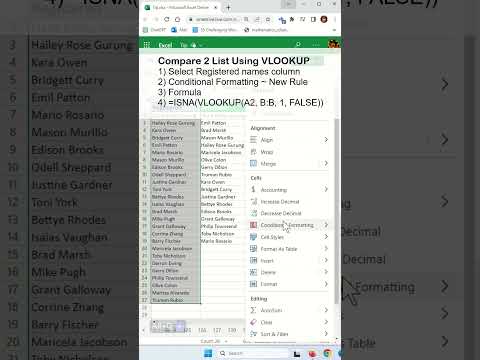 65,504 Views |
Essentially using VLOOKUP to compare two columns for matches, or in other words, compare two lists to find missing values using VLOOKUP in excel multiple. Some people like to use VLOOKUP to find missing data in two columns, like I’m demonstrating in this video. Also, they like to compare two columns in excel using VLOOKUP and return a third value. But in a nutshell, I’m using the VLOOKUP to compare two lists. And compare two columns and find missing values in excel.
Ok let answer this question, how to do a VLOOKUP in Excel to find missing data? Or how do you compare two lists in Excel to see if they match? Well…. you came to the right place, and this video explain just that.
These are the formulas outlined in this video.
1) Select Registered names column
2) Conditional Formatting ~ New Rule
3) Formula
4) =ISNA(VLOOKUP(A2, B:B, 1, FALSE))
Lets break down the formula.
VLOOKUP(A2, B:B, 1, FALSE): This is the inner function that performs the VLOOKUP operation. It searches for the value in cell A1 (the name from TABLE A) within the range B:B (the column of names in TABLE B) and returns the corresponding value from the first column (1) of that range. The last argument, FALSE, ensures an exact match is required.
ISNA(VLOOKUP(A1, B:B, 1, FALSE)): This formula wraps the VLOOKUP function with the ISNA function. ISNA stands for /”is not available/” and is used to check if the result of the VLOOKUP is #N/A, which indicates that the value in A1 was not found in the range B:B (i.e., the name from TABLE A is not present in TABLE B).
If the VLOOKUP returns #N/A, indicating that the name in A1 is not found in TABLE B, ISNA will return TRUE.
If the VLOOKUP returns a value (a match is found), ISNA will return FALSE.
Essentially, the formula ISNA(VLOOKUP(A1, B:B, 1, FALSE)) checks if the name in A1 exists in TABLE B. If it does not exist, it returns TRUE, indicating that the name is in TABLE A but not in TABLE B. If it does exist, it returns FALSE.
Alternatively, you can use this method.
1) Select Registered names column
2) Conditional Formatting ~ New Rule
3) Formula
4) =LEN(XLOOKUP(A2, B:B, B:B, /”/
Please take the opportunity to connect and share this video with your friends and family if you find it useful.


