
| Channel | Publish Date | Thumbnail & View Count | Actions |
|---|---|---|---|
 Rabi Gurung Rabi Gurung | 2023-10-12 14:38:00 | 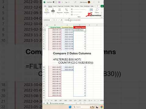 8,393 Views |
Comparing date columns in Excel can be a valuable task, particularly when working with large datasets or tracking time-sensitive information. To compare date columns, you can employ various methods depending on your specific needs. For example, to compare dates in Excel with the current date, you can use functions like /”TODAY()/” or /”NOW()/” to retrieve the current date or date and time, respectively. Then, you can use simple mathematical operators to check if a date in your column is equal to, greater than, or less than the current date. Additionally, when comparing two date-time values in Excel, you can use arithmetic operations to find the difference between the two and determine which one is more recent. Excel provides a versatile set of tools to help you effectively manage and analyze date-related data, making these comparisons an essential skill for many professionals and Excel users.
Use this formula as shown in my video.
=FILTER(B2:B30,NOT(COUNTIF(C2:C19,B2:B30)))
Here’s a breakdown of the formula step by step:
1) FILTER(B2:B30, …)
This part of the formula starts with the FILTER function, which is used to filter values from a range (in this case, B2:B30).
2) COUNTIF(C2:C19, B2:B30)
COUNTIF is an Excel function used to count the number of cells in a range that meet a specified condition.
In this case, it counts how many times each value in the range B2:B30 appears in the range C2:C19.
3) NOT(…)
The NOT function is used to reverse the logical result of the expression inside the parentheses.
So, NOT(COUNTIF(C2:C19, B2:B30)) will return TRUE if the value in B2:B30 does not appear in C2:C19 and FALSE if it does.
4) FILTER(B2:B30, NOT(…))
The FILTER function then filters the values in the range B2:B30 based on the condition specified in the NOT(COUNTIF(…)) part.
It returns only the values in B2:B30 for which the condition is TRUE (i.e., they do not appear in C2:C19).
In summary, this formula filters values from the range B2:B30 based on the condition that they do not appear in the range C2:C19. It returns a list of unique values from B2:B30 that are not found in C2:C19.
NOTE:
If you are getting 44879, that is actually the number so days since 1st January 1900.
LINKS TO SIMILIAR VIDEOS
How to compare two lists to find missing values WITHOUT FORMULA in excel – Excel Tips and Trick
https://youtube.com/shorts/pJtB8dbbimw?si=iL8qnDJ_WVAhKhAX
Compare two lists to find missing values using XLOOKUP in Excel – Excel Tips and Tricks
https://youtube.com/shorts/nOwMXkZJ5HU?si=N80igNW7Vr-xCK5x
Compare two lists to find missing values using VLOOKUP in Excel – Excel Tips and Tricks
https://youtube.com/shorts/1XGIPzsvS_Y?si=cu3ajNdT3lXFX3LB
How to compare two lists in Excel using Conditional Formatting – Excel Tips and Tricks
https://youtube.com/shorts/GX-BYEgcnRA?si=16oLe6kcxZExM4Df
How to compare two lists to find missing values in excel – Excel Tips and Tricks
https://youtube.com/shorts/dl75Lz_jaPs?si=-UTAvmCRdTl6ZZgm
#tip #excel #microsoft #shorts #shortvideo #shortsvideo #howto #how #google
Please take the opportunity to connect and share this video with your friends and family if you find it useful.


