
| Channel | Publish Date | Thumbnail & View Count | Actions |
|---|---|---|---|
 Rabi Gurung Rabi Gurung | 2023-12-20 13:00:34 | 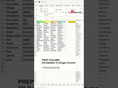 6,993 Views |
To compare multiple columns in Excel for matches, you can use various methods based on your specific requirements. If you aim to compare four columns, one approach involves using conditional formatting. Select the first column, go to /”Conditional Formatting,/” choose /”Highlight Cells Rules,/” and then opt for /”Duplicate Values./” This visually highlights matching values. For comparing multiple columns for matches, you can utilize functions like IF, COUNTIF, and AND to create custom formulas. If you’re specifically looking for an exact match between columns, you can employ the EXACT() function or use the = operator. To compare lists for matches in Excel, the VLOOKUP() or MATCH() functions can be useful, helping you identify commonalities or discrepancies between different sets of data.
The following formula convert 2 dimension array for dataset into a single column
=TOCOL(A2:D18)
Lets breakdown this formula.
=FILTER(UNIQUE(G2#), COUNTIF(G2#, UNIQUE(G2#)) > 1)
1) UNIQUE(G2#):
This part takes the range of values in column G (from cell G2 to the end of the data in column G, represented by G2#) and returns a list of unique values. It removes any duplicate values.
2) FILTER(UNIQUE(G2#), COUNTIF(G2#, UNIQUE(G2#)) > 1):
The FILTER function is used to filter the unique values obtained in step 1.
The condition for filtering is specified by COUNTIF(G2#, UNIQUE(G2#)) > 1. This condition checks how many times each unique value appears in the original range (G2#), and it only includes values that have a count greater than 1. In other words, it filters out values that are duplicated in the original range.
So, in summary, the entire formula filters out unique values from column G (excluding duplicates) that appear more than once in the original range. The result is a list of values that have duplicates in column G.
LINKS TO SIMILIAR VIDEOS
How to compare two lists to find missing values WITHOUT FORMULA in excel – Excel Tips and Trick
https://youtube.com/shorts/pJtB8dbbimw?si=iL8qnDJ_WVAhKhAX
Compare two lists to find missing values using XLOOKUP in Excel – Excel Tips and Tricks
https://youtube.com/shorts/nOwMXkZJ5HU?si=N80igNW7Vr-xCK5x
Compare two lists to find missing values using VLOOKUP in Excel – Excel Tips and Tricks
https://youtube.com/shorts/1XGIPzsvS_Y?si=cu3ajNdT3lXFX3LB
How to compare two lists in Excel using Conditional Formatting – Excel Tips and Tricks
https://youtube.com/shorts/GX-BYEgcnRA?si=16oLe6kcxZExM4Df
How to compare two lists to find missing values in excel – Excel Tips and Tricks
https://youtube.com/shorts/dl75Lz_jaPs?si=-UTAvmCRdTl6ZZgm
Excel Tips and Tricks – Compare Two Lists In Excel And Highlight
https://youtube.com/shorts/xJoy-nboV6A?feature=share
Summarize Duplicates in Excel – Excel Tips and Tricks
https://youtube.com/shorts/-IYUTWVmVTU?si=aN-hfbyQD0QEPcgm
Find difference quickly in Excel Comparing 2 List – Excel Tips and Tricks
https://youtube.com/shorts/8_-lN-yKf04?si=itTI-rcCKOaG7zVc
Compare multiple columns in Excel for matches – Excel Tips and Tricks
#shorts #microsoft #excel #microsoft #tiktok #shortvideo #howto #fyp #google
Please take the opportunity to connect and share this video with your friends and family if you find it useful.


